The ingenious Logarithm function

I always found it fascinating how so many Data Science algorithms are taking advantage of somehow simple mathematical concepts in order to achieve concrete goals. It is like using theoretical, abstract concepts and engineering them into something practical, effective and clever.

Some examples of these ideas are: the chain rule used in backpropagation; the sigmoid function (and similar), that is a bounded, differentiable and non-linear function used as an activation function; and exponential function, a differentiable function that allows to transform the inputs into positive numbers that can be summed up without cancelling out each others, in softmax function.

The question that recently came up to my mind was: Why is logarithm function so wildly used in Data Science? And what are the mysterious properties that make it so useful?

Lets try to solve this mystery.

Definition

The logarithm function states that if:

then \(y\) is the logarithm base \(a\) of \(x\):

In a simplified definition, the logarithm function compresses the range of large numbers and expands the range of small numbers.

It can be represented visually as shown in below plot.

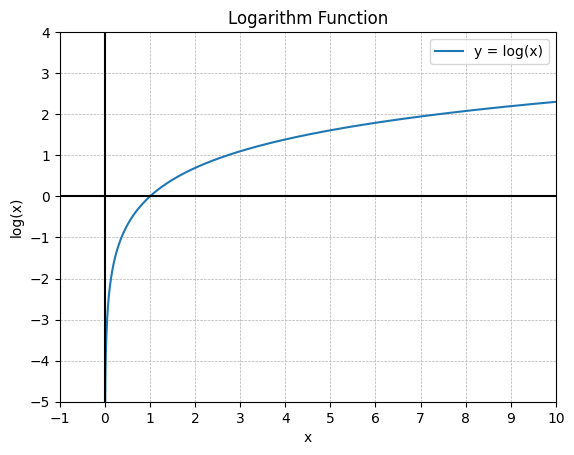
Fig. 01 - Logarithm function.

Properties

Lets take a look into some of \(log\) properties:

1. As described in the previous definition, logarithm is the inverse operation of exponential:

   \[\log_a x = y \implies a^y = x\]

2. With logarithm, powers become multiplications and multiplications become additions. These properties reduce the complexity of the computations:

   \[\log_a x^y = y\log_a x\] \[\log_a xy = \log_a x + \log_a b\]

3. It is a monotonic function, meaning that a larger value of \(x\) corresponds to a larger value of \(\log_a x\). These can be useful when optimizing a convex function, \(f(x)\), leading to:

   \[min(f(x)) = min(\log_a f(x))\] \[max(f(x)) = max(\log_a f(x))\]

4. The first and second derivatives of \(log\) can have much simpler computations. Especially in the case of the natural logarithm \(\ln\), for example:

   \[\frac{d}{dx} \ln x = \frac{1}{x}\]

Concrete Usage

Let’s now discuss some concrete examples of the logarithm use in Data Science.

Bar chart visualization

Have a look at the following bar graph:

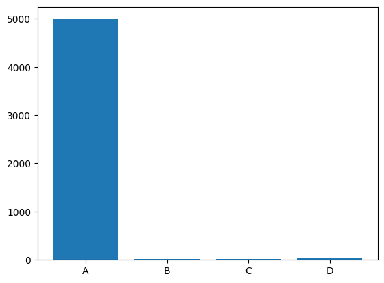
Fig. 02 - Bar chart where feature “A” has a bigger magnitude when compared with the other features.

In the bar chart above it is dificult to have a good overview about how features “B”, “C” and “D” relate to each other. The solution to this visualization problem is simple. We should apply the logarithm transformation to each of the features. In fact, matlibplot has this feature already built into the bar chart functionality, supported by parameter log = True.

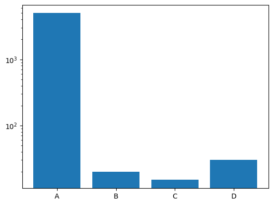
Fig. 03 - Bar chart with log = True.

Now it is easier to understand how features “B”, “C” and “D” relate to each other.

Right skewed distribution

Here is an example of a synthetic feature with a right skewed distribution.

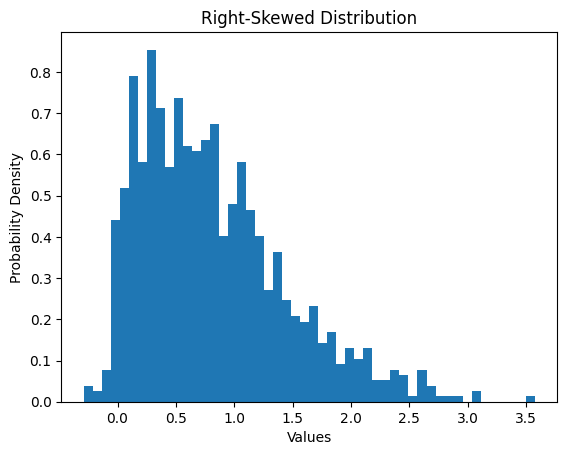
Fig. 04 - Right skewed distribution.

This feature has a heavy-tailed distribution that puts more probability mass in the tail range than a Gaussian distribution.

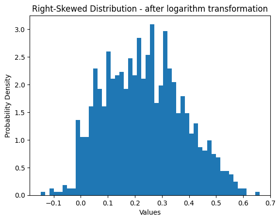
Fig. 05 - Right skewed distribution after logarithm transformation.

As it can be observed, after applying the logarithm function as a feature engineering procedure, the previously heavy-tailed distribution has now a near Gaussian distribution. It now compresses the long tail in the high end of the distribution into a shorter tail, and expands the short end into a longer head. This can be beneficial because many Machine Learning algorithms assume that the features are Gaussian distributed and perform better in this case.

The excellent book Feature Engineering for Machine Learning¹, by Alice Zheng and Amanda Casari, has an entire section dedicated to the log transformation. If you want to go deeper into these concepts, I highly recommend reading this book and more about the generalized power transformation.

Loss function

As you may already know, in order to optimize a Neural Network we need to minimize the loss function. From all the loss functions that we have available to solve classification problems, one is commonly used, the Negative Log-Likelihood.

Negative Log-Likelihood is defined as:

where \(y_i\) represents the probability score of the correct class, extracted from the softmax function.

But what does that mean? Why do we apply a logarithm function when calculating the loss?

It turns out that the Negative Log-Likelihood is one math trick used as a simplification to the real loss function that could have been used instead. We are talking about the Maximum Likelihood Estimation²:

This function estimates the parameters of a probability distribution that maximize the likelihood of the observed data. Check here³ to get a better understanding of the Maximum Likelihood Estimation.

But the former equation is prone to numerical underflow². Considering that the data is iid, and knowing that the \(\log\) of the likelihood does not affect the \(\operatorname{arg max}\), we can take advantage of it and transform it into:

This will protect the loss against numerical instability (underflow) and will result into better computation performance.

There is only one more step that needs to be done to land on the previously presented Negative log-Likelihood function. Because logarithm function is monotonic, likelihood and log-likelihood functions have the same extremum (\(max\) and \(min\) values), so maximizing the likelihood is the same as minimizing the Negative Log-Likelihood. As a consequence, the following expressions are equivalent, and we achieve our initial goal⁴:

It is important to understand that the logarithm function that is commonly used in Neural Networks is the \(\log_e\), also known as the natural logarithm \(\ln\). The preference for \(\ln\) is, most of the time, due to the use of the exponential function in the activation function of a previous layer, as for example, sigmoid, hyperbolic tangent and softmax functions. As previously mentioned, the logarithm function is the inverse operation of the exponential function, and when used together they cancel out each other:

Since the exponential function, in the activation function, can saturate when the inputs are very negative, the logarithm, in the loss function, reverses this effect.

Conclusion

The logarithm function has several valuable properties that make it very handy in data visualizations and when developing statistical and machine learning algorithms.

I hope this article helped you having a better understanding of the reasons to apply the logarithm function in Data Science, and maybe you can even take advantage of it in one of your next Data Science routines.

Please upvote or share this blog entry if you find it informative. Do not hesitate to comment below if you have questions, feedback or encouragement to give.

Remember, your voice matters.

References